Introduction
Installation
Note that ESBMTK 0.14.2.x requires python 3.12 or higher.
Conda
ESBMTK is available via the conda-forge channel https://conda-forge.org/ Assuming you install into a new virtual environment the following should install the ESBMTK framework
conda create --name foo python=3.12
conda activate foo
conda config --add channels conda-forge
conda config --set channel_priority strict
conda install esbmtk
pip & GitHub
If you work with pip, simply install with python -m pip install esbmtk, or download the code from https://github.com/uliw/esbmtk
A simple example
A simple model of the marine P-cycle would consider the delivery of P from weathering, the burial of P in the sediments, the thermohaline transport of dissolved PO4as well as the export of P in the form of sinking organic matter (POP). The concentration in the respective surface and deep water boxes is then the sum of the respective fluxes (see Fig. 1). The model parameters are taken from Glover 2011, Modeling Methods in the Marine Sciences.
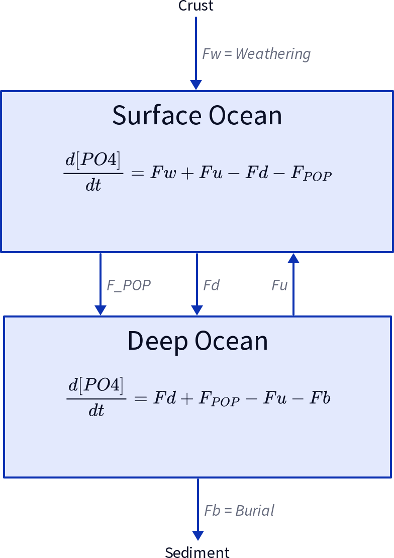
A two-box model of the marine P-cycle. Fw= weathering Fu= upwelling, Fd= downwelling, FPOP= particulate organic phosphor, Fb= burial.
If we define equations that control the export of particulate P (FPOP) as a fraction of the upwelling P (Fu), and the burial of P (Fb) as a fraction of (FPOP), we express this model as coupled ordinary differential equations (ODE, or initial value problem):
and for the deep ocean,
which is easily encoded as a Python function:
def dCdt(t, C_0, V, F_w, thx):
    """ Calculate the change in concentration as
    a function of time. After Glover 2011, Modeling
    Methods for Marine Science.

    :param C_0: tp.List of initial concentrations mol/m*3
    :param time: array of time points
    :params V: list of surface and deep ocean volume [m^3]
    :param F_w: River (weathering) flux of PO4 mol/s
    :param thx: thermohaline circulation in m*3/s
    :returns dCdt: tp.List of concentration changes mol/s
    """

    C_S = C_0[0]  # surface
    C_D = C_0[1]  # deep
    F_d = C_S * thx  # downwelling
    F_u = C_D * thx  # upwelling
    tau = 100 # residence time of P in surface waters [yrs]
    F_POP = C_S * V[0] / tau  # export production
    F_b = F_POP / 100  # burial

    dCdt[0] = (F_w + F_u - F_d - F_POP) / V[0]
    dCdt[1] = (F_d + F_POP - F_u - F_b) / V[1]

    return dCdt
Implementing the P-cycle with ESBMTK
While ESBMTK provides abstractions to efficiently define complex models, the following section will use the basic ESBMTK classes to define the above model. While quite verbose, it demonstrates the design philosophy behind ESBMTK. More complex approaches are described further down.
Foundational Concepts
- ESBMTK uses a hierarchically structured object-oriented approach to describe a model.
The topmost object is the model object that describes fundamental properties like run time, time step, elements and species information. All other objects derive from the model object. Reservoir objects define properties like volume or geometry, pressure and temperature, whereas species objects store initial conditions and concentration versus time data. Species Property objects store names and labels, and Element Property objects store e.g., isotopic reference ratios etc.
Model
   ├── Reservoir_1
   │   ├── Species_1
   │   │   └── SpeciesProperties
   │   │       └── ElementProperties
   │   └── Species_2
   │       └── SpeciesProperties
   │           └── ElementProperties
   └── Reservoir_2
       ├── Species_1
       │   └── SpeciesProperties
       │       └── ElementProperties
       └── Species_2
           └── SpeciesProperties
               └── ElementProperties
The relationship between two reservoirs is specified by a connection properties object that specifies which reservoir is the upstream source, and which is the downstream sink. It also specifies the type of connection, e.g., to scale the flux between from upstream to downstream by the respective species concentrations.
Model
   └── ConnectionProperties
       ├── Species2Species_1
       │   ├── Sink
       │   │   └── Reservoir
       │   │       └── Species_1
       │   ├── Source
       │   │   └── Reservoir
       │   │       └── Species_1
       │   └── Type
       │       └── ProcessProperties
       └── Species2Species_2
           ├── Sink
           │   └── Reservoir
           │       └── Species_2
           ├── Source
           │   └── Reservoir
           │       └── Species_2
           └── Type
               └── ProcessProperties
The model geometry is then parsed to build a suitable equation system which is passed to an ODE solver library which returns the results once integration has finished. Since Python objects are persistent, the object hierarchy is open to introspection using the regular Python syntax.
Defining the model geometry and initial conditions
The below code examples are available at https://github.com/uliw/esbmtk-examples In the first step, one needs to define a model object that describes fundamental model parameters. The following code first loads the following ESBMTK classes that will help with model construction:
esbmtk.base_classes.Reservoir()esbmtk.base_classes.SourceProperties()classesbmtk.base_classes.SinkProperties()classand
Q_which belongs to the pint library.
# import classes from the esbmtk library
from esbmtk import (
    Model,  # the model class
    Reservoir,  # the reservoir class
    ConnectionProperties,  # the connection class
    SourceProperties,  # the source class
    SinkProperties,  # sink class
)
Next we use the esbmtk.model.Model() class to create a model instance that defines basic model properties. Note that units are automatically translated into model units. While convenient, there are some important caveats:
Internally, the model uses ‘year’ as the time unit, mol as the mass unit, and liter as the volume unit. You can change this by setting these values to e.g., ‘mol’ and ‘kg’, however, some functions assume that their input values are in ‘mol/kg’ rather than mol/m**3 or ‘kg/s’. Ideally, this would be caught by ESBMTK, but at present, this is not guaranteed. So your mileage may vary if you fiddle with these settings. Note: Using mol/kg e.g., for seawater, will be discussed below.
# define the basic model parameters
M = Model(
    stop="3 Myr",  # end time of model
    max_timestep="1 kyr",  # upper limit of time step
    element=["Phosphor"],  # list of element definitions
)
Next, we need to declare some boundary conditions. Most ESBMTK classes will be able to accept input in the form of strings that also contain units (e.g., "30 Gmol/a" ). Internally these strings are parsed and converted into the model base units. This works most of the time, but not always. In the below example, we define the residence time \(\tau\). This variable is then used as input to calculate the scale for the primary production as M.S_b.volume / tau which must fail since M.S_b.volume is a numeric value and tau is a string.
# try the following
tau = "100 years"
tau * 12
To avoid this we have to manually parse the string into a quantity. This is done with the quantity operator Q_ Note that Q_ is not part of ESBMTk but imported from the pint library.
# now try this
from esbmtk import Q_
tau = Q_("100 years")
tau * 12
Most ESBMTK classes accept quantities, strings that represent quantities, as well as numerical values. Weathering and burial fluxes are often defined in mol/year, whereas ocean models use kg/year. ESBMTK provides a method (set_flux() ) that will automatically convert the input into the correct units. In this example, it is not necessary since the flux and the model both use mol. It is however good practice to rely on the automatic conversion. Note that it makes a difference for the mol to kilogram conversion whether one uses M.P or M.PO4 as the reference species!
# boundary conditions
F_w =  M.set_flux("45 Gmol", "year", M.P) # P @280 ppm (Filipelli 2002)
tau = Q_("100 year")  # PO4 residence time in surface box
F_b = 0.01  # About 1% of the exported P is buried in the deep ocean
thc = "20*Sv"  # Thermohaline circulation in Sverdrup
To set up the model geometry, we first use the esbmtk.base_classes.Source() and esbmtk.base_classes.Species() classes to create a source for the weathering flux, a sink for the burial flux, and instances of the surface and deep ocean boxes. Since we loaded the element definitions for phosphor in the model definition above, we can directly refer to the “PO4” species in the reservoir definition.
# Source definitions
SourceProperties(
    name="weathering",
    species=[M.PO4],
)
SinkProperties(
    name="burial",
    species=[M.PO4],
)
# reservoir definitions
Reservoir(
    name="S_b",  # box name
    volume="3E16 m**3",  # surface box volume
    concentration={M.PO4: "0 umol/l"},  # initial concentration
)
Reservoir(
    name="D_b",  # box name
    volume="100E16 m**3",  # deeb box volume
    concentration={M.PO4: "0 umol/l"},  # initial concentration
)
Model processes
For many models, processes can mapped as the transfer of mass from one box to the next. Within the ESBMTK framework, this is accomplished through the esbmtk.connections.Species2Species() class or the esbmtk.connections.ConnectionProperties() class. To connect the weathering flux from the source object (M.weathering) to the surface ocean (M.Sb) we declare a connection instance describing this relationship as follows:
ConnectionProperties(
    source=M.weathering,  # source of flux
    sink=M.S_b,  # target of flux
    rate=F_w,  # rate of flux
    id="river",  # connection id
    ctype="regular", #connection type
)
Unless the register keyword is given, connections will be automatically registered with the parent of the source, i.e., the model M. Unless explicitly given through the name keyword, connection names will be automatically constructed from the names of the source and sink instances. However, it is a good habit to provide the id keyword to keep connections separate in cases where two reservoir instances share more than one connection. The list of all connection instances can be obtained from the model object (see below).
The connection type ctype = "regular" or ctype = "fixed" is used when connecting reservoirs with a fixed rate (eg: Fw= 45 Gmol/year, as defined above). However, we may also create a concentration-dependent flux connection. To map the process of thermohaline circulation, for example, we connect the surface and deep ocean boxes using a connection type that scales the mass transfer as a function of the concentration in a given reservoir (ctype ="scale_with_concentration" ).
The concentration data is taken from the reference reservoir, which by default is the source reservoir. As such, in most cases, the ref_reservoirs keyword can be omitted. Note that the connection class does not require the name keyword. Rather, the name is derived from the source and sink reservoir instances. Since reservoir instances can have more than one connection (i.e., surface to deep via downwelling, and surface to deep via primary production), it is required to set the id keyword.
ConnectionProperties(  # thermohaline downwelling
    source=M.S_b,  # source of flux
    sink=M.D_b,  # target of flux
    ctype="scale_with_concentration",
    scale=thc, #(in sverdrups, i.e. volumetric rate)
    #volume / time * concentration (i.e. mass per unit volume) = flux (i.e. mass transfer per unit time)
    id="downwelling_PO4",
)
ConnectionProperties(  # thermohaline upwelling
    source=M.D_b,  # source of flux
    sink=M.S_b,  # target of flux
    ctype="scale_with_concentration",
    scale=thc,
    id="upwelling_PO4",
)
As seen above, the scale keyword can be a string or a numerical value. If it is provided as a string, ESBMTK will map the value into model units, i.e., the toolkit automatically handles unit conversions when scaling. For example, if concentration is described in mol/kg instead of mol/l, the above code for thermohaline circulation will automatically use the density of the relevant reservoirs to calculate the correct flux.
There are several ways to define biological export production, e.g., as a function of the upwelling PO4, or as a function of the residence time of PO4in the surface ocean. Here we follow Glover (2011) and use the residence time \(\tau\) = 100 years. Note that the below code species explicitly specifies the species that is affected by this process.
ConnectionProperties(  #
    source=M.S_b,  # source of flux
    sink=M.D_b,  # target of flux
    ctype="scale_with_concentration",
    scale=M.S_b.volume / tau,
    # volume / time * concentration (i.e. mass per unit volume) = flux (i.e mass transfer per unit time)
    id="primary_production",
    species=[M.PO4],  # apply this only to PO4
)
We require one more connection to describe the burial of P in the sediment. We describe this flux as a fraction of the primary export productivity. To create the connection we can either recalculate the export productivity or use the previously calculated flux via ctype ="scale_with_flux" and ref_flux.
ConnectionProperties(  #
    source=M.D_b,  # source of flux
    sink=M.burial,  # target of flux
    ctype="scale_with_flux",
    ref_flux="primary_production",
    scale=F_b,
    id="burial",
    species=[M.PO4],
)
Note that it is currently not possible to chain scale_with_flux references, e.g., referencing f1 to calculate f2 will work, but referencing f2 to calculate f3 will fail. Rather, calculate f3 from f1.
Running the above code (see the file po4_1.py at https://github.com/uliw/ESBMTK-Examples) and results in the following graph:

Example output from po4_1.png
Working with the model instance
Running the model, visualizing and saving the results
To run the model, use the run() method of the model instance, and plot the results with the plot() method. This method accepts a list of ESBMTK instances, that will be plotted in a common window. Without further arguments, the plot will also be saved as a pdf file where filename defaults to the name of the model instance. The save_data() method will create (or recreate) the data directory which will then be populated by csv-files.
M.plot([M.S_b.PO4, M.D_b.PO4], fn="po4_1.png")
# optionally, save data
# M.save_data(directory="./po4_1_data")
Saving/restoring the model state
Many models require a spin-up phase. Once the model is in equilibrium, you can save the save the state with the save_state() method.
M.run()
M.save_state()
Restarting the model from a saved state requires that you first initialize the model geometry (i.e., declare all the connections etc), and then read the previously saved model state.
....
....
M.read_state()
M.run()
Towards this end, note that a repeated model run will not be initialized from the last known state, but rather starts from a blank state.
.....
.....
M.run()
To restart a model from the last known state, the above would need to be written as
.....
.....
M.run()
M.save_state()
M.read_state()
M.run()
Introspection and data access
All ESBMTK instances and instance methods support the usual python methods to show the documentation, and inspect object properties.
help(M.S_b)  # will print the documentation for sb
dir(M.S_b)  # will print all methods for sb
M.S_b #  when issued in an interactive session, this will echo
# the arguments used to create the instance
The concentration data for a given reservoir is stored in the following instance variables:
M.S_b.c  # concentration
M.S_b.m  # mass
M.S_b.v  # volume
M.S_b.d  # delta value (if used by model)
M.S_b.l  # the concentration of the light isotope (if used)

# Appending _u will pprovide the data with units. This currently works for
M.S_b.c_u  # concentration
M.S_b.m_u  # mass
M.S_b.v_u  # volume
M.time_u # time
The model time axis is available as M.time and the model supports the esbmtk.model.Model.connection_summary() and esbmtk.model.Model.flux_summary()
# run tests
@pytest.mark.parametrize("test_input, expected", test_values)
def test_values(test_input, expected):
    t = 1e-4
    assert abs(expected) * (1 - t) <= abs(test_input) <= abs(expected) * (1 + t)