Adding Complexity

Model forcing

ESBMTK realizes model forcing through the esbmtk.extended_classes.Signal() class. Once defined, a signal instance can be associated with a esbmtk.connections.Species2Species() instance that will then act on the associated connection. This class provides the following keywords to create a signal:

• square(), pyramid(), bell() These are defined by specifying the signal start time (relative to the model time), its size (as mass) and duration, or as duration and magnitude (see the example below)

• filename() a string pointing to a CSV file that specifies the following columns: Time [yr], Rate/Scale [units], delta value [dimensionless] The class will attempt to convert the data into the correct model units. This process is however not very robust.

The default is to add the signal to a given connection. It is however also possible to use the signal data as a scaling factor. Signals are cumulative, i.e., complex signals are created by adding one signal to another (i.e., Snew = S1 + S2). Using the P-cycle model from the previous chapter (see po4_1.py) we can add a signal by first defining a signal instance, and then associating the instance with a weathering connection instance (this model is available as po4_2.p4 see https://github.com/uliw/ESBMTK-Examples)

from esbmtk import Signal

Signal(
    name="CR",  # Signal name
    species=M.PO4,  # SpeciesProperties
    start="1 Myrs",
    shape="pyramid",
    duration="1 Myrs",
    mass="45 Pmol",
)

ConnectionProperties(
    source=M.weathering,  # source of flux
    sink=M.S_b,  # target of flux
    rate=F_w,  # rate of flux
    id="river",  # connection id
    signal=M.CR,
    species=[M.PO4],
    ctype="regular",
)
M.run()

Note that the plot() method accepts the signal object as well. In general, any ESBMTK object that has data that varies with time, can be plotted by the plot() method. ESBMTK also provides classes to include external data esbmtk.extended_classes.ExternalData() as well as classes to mix and match data into the same plot esbmtk.extended_classes.DataField(). The file is92a_comparison_plots.py (see https://github.com/uliw/ESBMTK-Examples/tree/main/Boudreau/2010) shows a use case. Furthermore, esbmtk.model.Model.plot() returns a tuple with the figure instance, list of axs objects, which allows even more complex figure manipulations (see steady_state_plots.py in the same repository).

M.plot([M.S_b.PO4, M.D_b.PO4, M.CR], fn="po4_2.png")
#  M.save_data()

This will result in the following output:

Example output for the CR signal above. See po4_2.py in the examples directory.

Signal data structure

The original signal data (as read from a csv etc.) is available through the .s_time, .s_data instance variables. The padded/cropped data that is interpolated for each time point, is stored in the .cd_m (and .cd_l if isotope data is present) instance variables.The sub-sampled signal data that is used for plotting is stored in .m, .l and .d respectively. Signal data can also be queried interactively by calling the signal with a given time values, e.g., M.PO4_signal(12).

Working with multiple species

The basic building blocks introduced so far are sufficient to create a single species model. Adding further species is straightforward. First one needs to import the species definitions. They than can be simply used by extending the dictionaries and lists used in the previous example. Using the previous example of a simple P-cycle model, we now express the P-cycling as a function of photosynthetic organic matter (OM) production and remineralization. First, we import the new classes and we additionally load the species definitions for carbon (this code is available as po4_3.py see https://github.com/uliw/ESBMTK-Examples).

from esbmtk import (
    Model,
    Reservoir,  # the reservoir class
    ConnectionProperties,  # the connection class
    SourceProperties,  # the source class
    SinkProperties,  # sink class
    data_summaries,
    Q_,
)
M = Model(
    stop="6 Myr",  # end time of model
    max_timestep="1 kyr",  # upper limit of time step
    element=["Phosphor", "Carbon"],  # list of species definitions
)

# boundary conditions
F_w_PO4 =  M.set_flux("45 Gmol", "year", M.PO4) # P @280 ppm (Filipelli 2002)
tau = Q_("100 year")  # PO4 residence time in surface boxq
F_b = 0.01  # About 1% of the exported P is buried in the deep ocean
thc = "20*Sv"  # Thermohaline circulation in Sverdrup
Redfield = 106 # C:P

SourceProperties(
    name="weathering",
    species=[M.PO4, M.DIC],
)
SinkProperties(
    name="burial",
    species=[M.PO4, M.DIC],
)
Reservoir(
    name="S_b",
    volume="3E16 m**3",  # surface box volume
    concentration={M.DIC: "0 umol/l", M.PO4: "0 umol/l"},
)
Reservoir(
    name="D_b",
    volume="100E16 m**3",  # deep box volume
    concentration={M.DIC: "0 umol/l", M.PO4: "0 umol/l"},
)

The esbmtk.connections.ConnectionProperties.() class definition is equally straightforward, and the following expression will apply the thermohaline downwelling to all species in the M.S_b group.

ConnectionProperties(  # thermohaline downwelling
    source=M.S_b,  # source of flux
    sink=M.D_b,  # target of flux
    ctype="scale_with_concentration",
    scale=thc,
    id="thc_up",
)
ConnectionProperties(  # thermohaline upwelling
    source=M.D_b,  # source of flux
    sink=M.S_b,  # target of flux
    ctype="scale_with_concentration",
    scale=thc,
    id="thc_down",
)

It is also possible to specify individual rates or scales using a dictionary, as in this example that sets two different weathering fluxes:

ConnectionProperties(
    source=M.weathering,  # source of flux
    sink=M.S_b,  # target of flux
    rate={M.DIC: F_w_PO4 * Redfield, M.PO4: F_w_PO4},  # rate of flux
    ctype="regular",
    id="weathering",  # connection id
)

The following code defines primary production and its effects on DIC in the surface and deep box. The example is a bit contrived but demonstrates the principle. Note the use of the ref_reservoirs keyword and Redfield ratio

# P-uptake by photosynthesis
ConnectionProperties(  #
    source=M.S_b,  # source of flux
    sink=M.D_b,  # target of flux
    ctype="scale_with_concentration",
    scale=M.S_b.volume / tau,
    id="primary_production",
    species=[M.PO4],  # apply this only to PO4
)
# OM Primary production as a function of P-concentration
ConnectionProperties(  #
    source=M.S_b,  # source of flux
    sink=M.D_b,  # target of flux
    ref_reservoirs=M.S_b.PO4,
    ctype="scale_with_concentration",
    scale=Redfield * M.S_b.volume / tau,
    species=[M.DIC],
    id="OM_production",
)
# P burial
ConnectionProperties(  #
    source=M.D_b,  # source of flux
    sink=M.burial,  # target of flux
    ctype="scale_with_flux",
    ref_flux=M.flux_summary(filter_by="primary_production",return_list=True)[0],
    scale={M.PO4: F_b, M.DIC: F_b * Redfield},
    id="burial",
)

One can now proceed to define the particulate phosphate transport as a function of organic matter export

M.run()
pl = data_summaries(
    M,  # model instance
    [M.DIC, M.PO4],  # SpeciesProperties list
    [M.S_b, M.D_b],  # Reservoir list
)
M.plot(pl, fn="po4_3.png")

which results in the below plot. The full code is available in the examples directory as po4_2.py

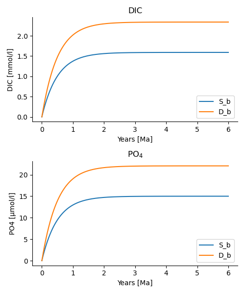
Output of po4_3.py demonstrating the use of the data_summaries() function

Using many boxes

Using the ESBMTK classes introduced thus far is sufficient to build complex models. However, it is beneficial to leverage Python syntax to create utility functions that help reduce overly verbose code. The ESBMTK library includes several routines that aid in this process; however, they are not part of the core API, are not yet well documented, and have not undergone extensive testing. The following provides a brief introduction, but it may be useful to examine the code for the Boudreau 2010 model in the example directory, as it makes significant use of the Python dictionary class.

For these functions to operate correctly, box names must adhere to the following template: Area_depth, such as L_sb for a low latitude surface water box or D_db for a deep water box. While the actual names are flexible, the underscore is utilized to distinguish between ocean area (eg. low-latitude, high-latitude, etc.) and depth interval (eg. surface, intermediate, deep, etc.).

The following code examples demonstrate how to create multiple boxes simultaneously by first defining a dictionary containing the box geometry and initial values, followed by the esbmtk.utility_functions.initialize_reservoirs() function to instantiate the corresponding Reservoir objects. The Boudreau2010.py example available at https://github.com/uliw/ESBMTK-Examples illustrates a practical application of this approach.

box_parameters: dict = {  # name: [[geometry], T, P]
    "H_b": {  # High-Lat Box
        "c": {
            M.DIC: "2153 umol/kg",
            M.TA: "2345 umol/kg",
            M.PO4: "1.5 umol/kg",
            M.O2: "200 umol/kg",
        },
        "g": {"area": "0.5e14m**2", "volume": "1.76e16 m**3"},  # geometry
        "T": 2,  # temperature in C
        "P": 17.6,  # pressure in bar
        "S": 35,  # salinity in psu
    },
    "L_b": {  # Low-Lat Box
        "c": {
            M.DIC: "1952 umol/kg",
            M.TA: "2288 umol/kg",
            M.PO4: "1.5 umol/kg",
            M.O2: "200 umol/kg",
        },
        "g": {"area": "2.85e14m**2", "volume": "2.85e16 m**3"},
        "T": 21.5,
        "P": 5,
        "S": 35,
    },
# Instantiate Reservoir objects
species_list = initialize_reservoirs(M, box_parameters)

Similarly, we can leverage Python dictionaries to set up the transport matrix. The dictionary key must use the following template: boxname_to_boxname@id where the id is used similarly to the connection id in the Species2Species and ConnectionProperties classes.

So to specify, for example, thermohaline upwelling from the Atlantic deep water to the Atlantic intermediate water, you would use A_db_to_A_ib@thc as the dictionary key, followed by the rate. The following examples define the thermohaline transport in a LOSCAR-type model (based on https://gmd.copernicus.org/articles/5/149/2012/):

# Conveyor belt
thc = Q_("20*Sv")
ta = 0.2  # upwelling coefficient Atlantic ocean
ti = 0.2  # upwelling coefficient Indian ocean

# Specify the mixing and upwelling terms as dictionary
thx_dict = {  # Conveyor belt
    "H_sb_to_A_db@thc": thc,
    # Upwelling
    "A_db_to_A_ib@thc": ta * thc,
    "I_db_to_I_ib@thc": ti * thc,
    "P_db_to_P_ib@thc": (1 - ta - ti) * thc,
    "A_ib_to_H_sb@thc": thc,
    # Advection
    "A_db_to_I_db@adv": (1 - ta) * thc,
    "I_db_to_P_db@adv": (1 - ta - ti),
    "P_ib_to_I_ib@adv": (1 - ta - ti),
    "I_ib_to_A_ib@adv": (1 - ta) * thc,
}

to create the actual connections we need to:

1. Assemble a list of all species that are affected by thermohaline circulation

2. Specify the connection type that describes thermohaline transport, i.e., scale_by_concentration

3. Combine #1 & #2 into a dictionary that can be used by the create_bulk_connections() function to instantiate the necessary connections.

species_names = list(ic.keys())  # get species list
connection_type = {"ty": "scale_with_concentration", "sp": sl}
connection_dictionary = build_ct_dict(thx_dict, species_names)
create_bulk_connections(connection_dictionary, M, mt="1:1")

In the following example, we build the connection_dictionary in a more explicit way to define primary production as a function of P upwelling: the first line finds all the upwelling fluxes, and we can then use them as an argument in the connection_dictionary definition:

# get all upwelling P fluxes except for the high latitude box
pfluxes = M.flux_summary(filter_by="PO4_mix_up", exclude="H_", return_list=True)

# define export productivity in the high latitude box
PO4_ex = Q_(f"{1.8 * M.H_sb.area/M.PC_ratio} mol/a") #PC ratio = Phosphorus:Carbon ratio

c_dict = {  # Surface box to ib, about 78% is remineralized in the ib
    ("A_sb_to_A_ib@POM_P", "I_sb_to_I_ib@POM_P", "P_sb_to_P_ib@POM_P"): {
        "ty": "scale_with_flux",
        "sc": M.PUE * M.ib_remin, #PUE = Phosphorus Utilization Efficiency
        "re": pfluxes,
        "sp": M.PO4,
    },  # surface box to deep box
    ("A_sb_to_A_db@POM_P", "I_sb_to_I_db@POM_P", "P_sb_to_P_db@POM_P"): {
        "ty": "scale_with_flux",
        "sc": M.PUE * M.db_remin,
        "re": pfluxes,
        "sp": M.PO4,
    },  # high latitude box to deep ocean boxes POM_P
    ("H_sb_to_A_db@POM_P", "H_sb_to_I_db@POM_P", "H_sb_to_P_db@POM_P"): {
        # here we use a fixed rate following Zeebe's Loscar model
        "ra": [
            PO4_ex * 0.3,
            PO4_ex * 0.3,
            PO4_ex * 0.4,
        ],
        "sp": M.PO4,
        "ty": "Fixed",
    },
}
create_bulk_connections(c_dict, M, mt="1:1")

In the last example, we use the gen_dict_entries function to extract a list of connection keys that can be used in the connection_dictionary . The following code finds all connection keys that match the particulate organic phosphor fluxes (POM_P) defined in the code above, and to replace them with a connection key that uses POM_DIC as id-string. The function returns a list of fluxes and matching keys that can be used to specify new connections. See also boudreau2010.py which uses a less complex setup (https://github.com/uliw/ESBMTK-Examples).

keys_POM_DIC, ref_fluxes = gen_dict_entries(M, ref_id="POM_P", target_id="POM_DIC")

c_dict = {
    keys_POM_DIC: {
        "re": ref_fluxes,
        "sp": M.DIC,
        "ty": "scale_with_flux",
        "sc": M.PC_ratio,
        "al": M.OM_frac,
    }
}
create_bulk_connections(c_dict, M, mt="1:1")